spin – expploration

Some particles have helicity, some have spin

Photons and Neutrinos have helicity while Electrons and Muons have spin. In general, a massless particle has a helicity while a massive particle has spin. In this post, I want to explore the peculiarities of the massive and the massless case which results in this difference.

Spin is a characteristic quantum numbers

Any free particle has a momentum and a set of other characteristics. An electron, for example, has a momentum, a characteristic mass, a characteristic charge etc. Spin is, likewise, a characteristic of a particle. An Electron always has spin $j = \frac{1}{2}$ , for example.

There exists something analogous to spin for Photons (not helicity) which we will explore in this post. There’s no name for this quantum number as it is always 0. However, we will see that just like a spin $\frac{1}{2}$ particle has two states $j_z = + \frac{1}{2}$ and $j_z = - \frac{1}{2}$ , similarly, Photons have two states with helicities +1 and -1. Therefore, helicity is analogous to the z component of spin and not spin itself.

Where do characteristic quantum numbers come from?

Any symmetry transformation will leave characteristic quantum numbers invariant. If it did not leave it invariant, then we would be able to change the measured charge of an electron by simply rotating our co-ordinate system, for example, which is ludicrous.

In group theoretic terms, this means that the operator, whose eigenvalue gives us the characteristic Quantum numbers, must commute with all generators of the symmetry group. Such operators are called Casimir operators.

The characteristic Quantum numbers are, therefore, Casimir operators corresponding to symmetries. In fact, both spin and helicity originate from the same Casimir operator. This is a Casimir operator of the Poincare group, which is a well known symmetry of nature,

Casimir operators of the Poincare group

The Poincare group has two Casimir operators: the well known $P^{\mu} P_{\mu}$ and the not so well known $W^{\mu}W_{\mu}$ , where $P$ is the four-momentum operator and $W$ is the Pauli-Lubansky four-vector given by the expression:

$W^{\mu} = -\frac{1}{2} \epsilon^{\mu\nu\rho\sigma}J_{\nu\rho}P_{\sigma}$

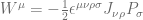
It turns out that spin is the quantum number corresponding to the Casimir operator $W^{\mu}W_{\mu}$ in the case of massive particles. In the case of massless particles $W^{\mu}W_{\mu}$ is taken to be zero. Let us discuss these two cases separately and see how this comes about.

Massive particles have spin

To evaluate the Casimir operator for massive particles, we go to the rest frame of the particle, where its momentum is $\left( m,0,0,0 \right)$ . In this frame, $W^0 = 0$ and $W^i = mJ^i$ and therefore:

$-W^{\mu}W_{\mu} = m^2 \mathbf{J}^2$

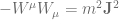
This looks like the familiar total spin angular momentum operator.The eigenvalue of $\mathbf{J}^2$ is $j(j+1)$ . Therefore massive particles are labeled by their spin value $j$ (which is the characteristic quantum number). States within each representation are labeled by the $j_z = -j, -j+1, \dots , j$ .

Therefore, a massive particle can be labeled by the following quantum numbers $m^2, j, p \textrm{ and } j_z$ .

One last comment before we close the section on massive particles: Note that we have derived the operators for a certain choice of momentum. These operators are going to look different for different choices of momentum. The Casimir operator will no longer look like $\mathbf{J^2}$ and $J_z$ is not going to look like $J_z$ . This is obvious as $J_z$ doesn’t even commute with momentum in general, it only commutes in this special case with a special choice of the momentum.

The subgroup of the Poincare group which keeps a certain choice of momentum unchanged is known as the ‘little group’. The operators that generate the little group commute with momentum and hence can be used to label particle states. $J_z$ is a generator of the little group which keeps the momentum $\left( m, 0, 0, 0 \right)$ unchanged and hence we could use it to label our states.

Massless particles are…umm…different

The situation is different for massless particles. The momentum of a massless particle in its rest frame can be written as $\left( \omega, 0, 0, \omega \right)$ . In this frame, a straightforward computation gives $W^0 = W^3 = \omega J^3$ , $W^1 = \omega \left( J^1 - K^2 \right) \equiv \omega A$ and $W^2 = \omega \left( J^2 + K^1 \right) \equiv \omega B$ . Therefore:

$-W_{\mu}W^{\mu} = \omega^2 \left[ \left( K^2 - J^1 \right)^2 + \left( K^1 + J^2 \right)^2 \right] = \omega \left[ A^2 + B^2 \right]$

These operators $A$ and $B$ , along with $J^3$ , close an algebra corresponding to the ‘little group’ in the massless case.

$\left[J^3,A \right] = iB, \; \left[ J^3, B \right] = -iA, \;\left[ A,B \right] = 0$

It turns out that $A$ and $B$ commute. Thus we can have states that are simultaneously eigenvalues of both operators.

$A \left| p; a,b \right> = a \left| p;a,b \right>, \; B \left| p;a,b \right> = b \left | p; a,b\right>$

On these states, we can evaluate the Casimir operator, which gives us the characteristic quantum number:

$-W^{\mu}W_{\mu} = \omega^2 ( a^2 + b^2 )$

But it doesn’t end there. To complicate matters, it turns out that if $\left| p;a,b \right>$ is an eigenstate of $A$ and $B$ , so is the state:

$\left| p,a,b,\theta \right> \equiv e^{-i\theta J^3} \left| p; a,b \right>$

On this state the eigenvalue of $A$ is $a(\theta) \equiv \left( a \cos \theta - b \sin \theta \right)$ and the eigenvalue of $B$ is $b(\theta) \equiv\left( a \sin \theta + b \cos \theta \right)$ !

This means that, unless $a=b=0$ , we find a states corresponding with a continuous internal degree of freedom $\theta$ ! These quantum numbers don’t seem to exist (find physical applications) in Nature. Thus we are forced to choose $a=b=0$ , which makes our Casimir operator zero.

$-W^{\mu} W_{\mu} = 0$

The analog of spin for a massless particle is therefore 0.

Massless particles have helicity

We found that the Casimir operator is zero for all massless particles. We still have to label the states though, like we did in the massive case. In order to do this, we need to find the maximal set of commuting operators. We already have $P^{\mu}P_{\mu}$ and $W^{\mu}W_{\mu}$ . We have found three operators $A$ , $B$ and $J^3$ , which commute with $P^{\mu}$ . Of course, the operator $A$ and $B$ cannot be used to label the states as we found that all their eigenvalues are zero. We can, however, try $J^3$ , which may give us non zero eigenvalues.

$J^3$ generates rotations in the x-y plane which correspond to an Abelian $SO(2)$ algebra. All irreducible representations of this Abelian group (or any Abelian group, for that matter) are one dimensional. Therefore, there is only one state in the representation.

The eigenvalue of $J^3$ on this one dimensional state is known as helicity. It can be shown (using topological arguments) that the eigenvalue is quantized and can take values $h = 0, \pm \frac{1}{2}, \pm 1, \dots$ .

Helicity and parity

We also remember that the choice of the momentum was arbitrary. We could have chosen the three momentum to be in any direction we wanted. Therefore, the following is a more general and accurate representation of the helicity operator:

$H = \hat{\mathbf{p}} \cdot \mathbf{J}$

From this expression we can immediately see that helicity is a pseudoscalar, i.e, it changes sign under a parity transformation. Thus, even though particles with $h = 1$ and $h= -1$ are logically two different species of particles under the Poincare algebra, parity exchanges them. If parity is a symmetry of the theory under consideration, then it is more convenient to group together particles with opposite parity and call them ‘left handed’ and ‘right handed’ variants of the same particle.

Parity is a symmetry of both electromagnetism and gravitation. Thus we have two polarization states of the Photon ( $h = \pm 1$ ) and two polarization states of the Graviton ( $h = \pm 2$ ). On the other hand, Neutrinos, which only interact via the parity violating weak interaction, are given different names according to their helicity. The name Neutrino is reserved for $h = -\frac{1}{2}$ and the name Antineutrino is reserved for $h = +\frac{1}{2}$ .

expploration

explore the world of elementary particle physics

Tag: spin

What the hell is helicity and how is it different from spin?