Theories of Everything, Mapped

LinkOctober 1, 2015October 1, 2015 dibyaLeave a comment

Explore the deepest mysteries at the frontier of fundamental physics, and the most promising ideas put forth to solve them. Source: Theories of Everything, Mapped

vector-scalar-complex-dirac-quantization

How to quantize a field?

September 24, 2015September 24, 2015 dibyaLeave a comment

In an earlier blog post, I shared a link to a mind map of important fields in relativistic field theory. In this mind map, we explored the classical field theory of scalar fields, complex scalar fields, Weyl spinors, Dirac spinors, Majorana spinors and the Vector field. Each of these fields correspond to a simple representation of the Lorentz group. A classical theory of these fields was the first step in going towards a Lorentz invariant theory of particles.

The next step involves going from classical fields to quantum particles. In order to do this, we need to make the fields operator valued and impose suitable commutation or anti-commutation relations on them. This is an elaborate endeavour in itself and hence I decided to dedicate another mind map to this process.

This mind map is about the Quantization of Fields and I am happy to share the link to it here:

https://coggle.it/diagram/VgFKcfyW5qwCs2Va/26b15bd0a9cc5ca6d4fc327af60f2c24fb3e6c5648a344b1840a47bb145e2a22

You may at any time create your own copy of this mind map and customize it for your study. Feel free to suggest changes as well. If you feel that I have missed an important sub-concept associated to the central concept of quantization, drop me a line and I will try my best to include it.

Thanks for your readership.

The bizarre parity transformation (in a mind map)

September 4, 2015September 24, 2015 dibyaLeave a comment

Parity is the operation of flipping the signs of odd numbers of space like co-ordinates.

parity-coordinate-flip — parity-transformation

The operation of parity is not made up of products of many infinitesimal operations starting from identity. It is a discrete transformation and fundamentally different from rotation.

The transformation of Quantum systems under the operation of parity can be quite bizarre. To add to our woes, it also turns out that under certain specific interactions, nature does not preserve parity of physical systems under time evolution! This is known as P violation or Parity violation.

I have summarized the amazing world of Parity in the context of Quantum systems in a mind map drawn in coggle. Take a look 🙂

https://embed.coggle.it/diagram/55e846396a271eae4c8e2d08/758bfbfd53d56bbed23f67acbde5dea16cab14735a38cb7be7d290c43790e888

What the hell is helicity and how is it different from spin?

September 1, 2015September 1, 2015 dibyaLeave a comment

Some particles have helicity, some have spin

Photons and Neutrinos have helicity while Electrons and Muons have spin. In general, a massless particle has a helicity while a massive particle has spin. In this post, I want to explore the peculiarities of the massive and the massless case which results in this difference.

Spin is a characteristic quantum numbers

Any free particle has a momentum and a set of other characteristics. An electron, for example, has a momentum, a characteristic mass, a characteristic charge etc. Spin is, likewise, a characteristic of a particle. An Electron always has spin $j = \frac{1}{2}$ , for example.

There exists something analogous to spin for Photons (not helicity) which we will explore in this post. There’s no name for this quantum number as it is always 0. However, we will see that just like a spin $\frac{1}{2}$ particle has two states $j_z = + \frac{1}{2}$ and $j_z = - \frac{1}{2}$ , similarly, Photons have two states with helicities +1 and -1. Therefore, helicity is analogous to the z component of spin and not spin itself.

Where do characteristic quantum numbers come from?

Any symmetry transformation will leave characteristic quantum numbers invariant. If it did not leave it invariant, then we would be able to change the measured charge of an electron by simply rotating our co-ordinate system, for example, which is ludicrous.

In group theoretic terms, this means that the operator, whose eigenvalue gives us the characteristic Quantum numbers, must commute with all generators of the symmetry group. Such operators are called Casimir operators.

The characteristic Quantum numbers are, therefore, Casimir operators corresponding to symmetries. In fact, both spin and helicity originate from the same Casimir operator. This is a Casimir operator of the Poincare group, which is a well known symmetry of nature,

Casimir operators of the Poincare group

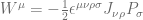
The Poincare group has two Casimir operators: the well known $P^{\mu} P_{\mu}$ and the not so well known $W^{\mu}W_{\mu}$ , where $P$ is the four-momentum operator and $W$ is the Pauli-Lubansky four-vector given by the expression:

$W^{\mu} = -\frac{1}{2} \epsilon^{\mu\nu\rho\sigma}J_{\nu\rho}P_{\sigma}$

It turns out that spin is the quantum number corresponding to the Casimir operator $W^{\mu}W_{\mu}$ in the case of massive particles. In the case of massless particles $W^{\mu}W_{\mu}$ is taken to be zero. Let us discuss these two cases separately and see how this comes about.

Massive particles have spin

To evaluate the Casimir operator for massive particles, we go to the rest frame of the particle, where its momentum is $\left( m,0,0,0 \right)$ . In this frame, $W^0 = 0$ and $W^i = mJ^i$ and therefore:

$-W^{\mu}W_{\mu} = m^2 \mathbf{J}^2$

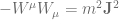
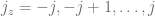
This looks like the familiar total spin angular momentum operator.The eigenvalue of $\mathbf{J}^2$ is $j(j+1)$ . Therefore massive particles are labeled by their spin value $j$ (which is the characteristic quantum number). States within each representation are labeled by the $j_z = -j, -j+1, \dots , j$ .

Therefore, a massive particle can be labeled by the following quantum numbers $m^2, j, p \textrm{ and } j_z$ .

One last comment before we close the section on massive particles: Note that we have derived the operators for a certain choice of momentum. These operators are going to look different for different choices of momentum. The Casimir operator will no longer look like $\mathbf{J^2}$ and $J_z$ is not going to look like $J_z$ . This is obvious as $J_z$ doesn’t even commute with momentum in general, it only commutes in this special case with a special choice of the momentum.

The subgroup of the Poincare group which keeps a certain choice of momentum unchanged is known as the ‘little group’. The operators that generate the little group commute with momentum and hence can be used to label particle states. $J_z$ is a generator of the little group which keeps the momentum $\left( m, 0, 0, 0 \right)$ unchanged and hence we could use it to label our states.

Massless particles are…umm…different

The situation is different for massless particles. The momentum of a massless particle in its rest frame can be written as $\left( \omega, 0, 0, \omega \right)$ . In this frame, a straightforward computation gives $W^0 = W^3 = \omega J^3$ , $W^1 = \omega \left( J^1 - K^2 \right) \equiv \omega A$ and $W^2 = \omega \left( J^2 + K^1 \right) \equiv \omega B$ . Therefore:

$-W_{\mu}W^{\mu} = \omega^2 \left[ \left( K^2 - J^1 \right)^2 + \left( K^1 + J^2 \right)^2 \right] = \omega \left[ A^2 + B^2 \right]$

These operators $A$ and $B$ , along with $J^3$ , close an algebra corresponding to the ‘little group’ in the massless case.

$\left[J^3,A \right] = iB, \; \left[ J^3, B \right] = -iA, \;\left[ A,B \right] = 0$

It turns out that $A$ and $B$ commute. Thus we can have states that are simultaneously eigenvalues of both operators.

$A \left| p; a,b \right> = a \left| p;a,b \right>, \; B \left| p;a,b \right> = b \left | p; a,b\right>$

On these states, we can evaluate the Casimir operator, which gives us the characteristic quantum number:

$-W^{\mu}W_{\mu} = \omega^2 ( a^2 + b^2 )$

But it doesn’t end there. To complicate matters, it turns out that if $\left| p;a,b \right>$ is an eigenstate of $A$ and $B$ , so is the state:

$\left| p,a,b,\theta \right> \equiv e^{-i\theta J^3} \left| p; a,b \right>$

On this state the eigenvalue of $A$ is $a(\theta) \equiv \left( a \cos \theta - b \sin \theta \right)$ and the eigenvalue of $B$ is $b(\theta) \equiv\left( a \sin \theta + b \cos \theta \right)$ !

This means that, unless $a=b=0$ , we find a states corresponding with a continuous internal degree of freedom $\theta$ ! These quantum numbers don’t seem to exist (find physical applications) in Nature. Thus we are forced to choose $a=b=0$ , which makes our Casimir operator zero.

$-W^{\mu} W_{\mu} = 0$

The analog of spin for a massless particle is therefore 0.

Massless particles have helicity

We found that the Casimir operator is zero for all massless particles. We still have to label the states though, like we did in the massive case. In order to do this, we need to find the maximal set of commuting operators. We already have $P^{\mu}P_{\mu}$ and $W^{\mu}W_{\mu}$ . We have found three operators $A$ , $B$ and $J^3$ , which commute with $P^{\mu}$ . Of course, the operator $A$ and $B$ cannot be used to label the states as we found that all their eigenvalues are zero. We can, however, try $J^3$ , which may give us non zero eigenvalues.

$J^3$ generates rotations in the x-y plane which correspond to an Abelian $SO(2)$ algebra. All irreducible representations of this Abelian group (or any Abelian group, for that matter) are one dimensional. Therefore, there is only one state in the representation.

The eigenvalue of $J^3$ on this one dimensional state is known as helicity. It can be shown (using topological arguments) that the eigenvalue is quantized and can take values $h = 0, \pm \frac{1}{2}, \pm 1, \dots$ .

Helicity and parity

We also remember that the choice of the momentum was arbitrary. We could have chosen the three momentum to be in any direction we wanted. Therefore, the following is a more general and accurate representation of the helicity operator:

$H = \hat{\mathbf{p}} \cdot \mathbf{J}$

From this expression we can immediately see that helicity is a pseudoscalar, i.e, it changes sign under a parity transformation. Thus, even though particles with $h = 1$ and $h= -1$ are logically two different species of particles under the Poincare algebra, parity exchanges them. If parity is a symmetry of the theory under consideration, then it is more convenient to group together particles with opposite parity and call them ‘left handed’ and ‘right handed’ variants of the same particle.

Parity is a symmetry of both electromagnetism and gravitation. Thus we have two polarization states of the Photon ( $h = \pm 1$ ) and two polarization states of the Graviton ( $h = \pm 2$ ). On the other hand, Neutrinos, which only interact via the parity violating weak interaction, are given different names according to their helicity. The name Neutrino is reserved for $h = -\frac{1}{2}$ and the name Antineutrino is reserved for $h = +\frac{1}{2}$ .

A mind map of Quantum Fields

August 28, 2015September 24, 2015 dibya3 Comments

What is a mind map?

A mind map is a diagram used for visually organizing connected information. A mind map often revolves around a central concept or idea which is represented at the centre of the diagram. The representation can be in the form of text, images, links equations etc. Associated ideas or concepts branch out from the central concept. The branching can go on indefinitely until all the information associated with the central concept has been represented on the diagram.

Mind maps make complicated ideas look simple by providing a bird’s eye view of the inter-relationship between a central idea and associated ideas. This helps in memorization, seeing the big pictures, and in some cases, connecting the dots.

Studying Quantum Field Theory can be frustrating

I had decided earlier that I would study Physics using mind maps at some point in my life. In particular, I was frustrated at my inability to memorize the concepts of Quantum field theory. QFT is a complex theory with hundreds of associated concepts which find application, not only in the theory of elementary particles, but also in Condensed matter physics and Cosmology. I also felt the need to eliminate the noise and look at the big picture at times. Therefore I decided to start making mind maps to make sense of things.

Mind mapping Quantum Fields with Coggle

Recently I came across Coggle, a beautiful web based mind mapper with LaTeX support and I decided to start making mind maps on QFT and Elementary Particle Physics.

I made a mind map on Quantum Fields and I wanted to share it on my blog. Here it is (still a bit incomplete though):

https://embed.coggle.it/diagram/55dc56db241048026b544f39/eba0b19af09909f844d1d3838c74de17bc8b050078d95bf10622c0224d14c8f3

Compton wavelength via dimensional analysis

August 12, 2015August 24, 2015 dibyaLeave a comment

Dimensional analysis is cool because it gets wonderful results out of literally nothing. In this post, we figure out the Compton wavelength of an electron by simply talking and doing little to zero maths.

The cool way of finding the Compton wavelength of an electron

Suppose we want to find the Compton wavelength of the electron.
We know that the Compton effect is seen when a photon scatters off an electron. Therefore the physical entities that play a role in Compton scattering are the electron and the photon. An electron has a fixed mass and charge. The photon has a fixed velocity. We argue, therefore, that the Compton wavelength, which is a fixed quantity, must depend on these other fixed quantities and nothing else.‘
We reduce the set of quantities that might make up the Compton wavelength by further noting that the Compton effect occurs because of relativistic energy momentum conservation in an inelastic scattering. Since the photon wavelength is determined purely by energy momentum conservation, the electric charge plays no role : it could have been anything and the results would have been the same. Also, we can forget about $c$ and $\hbar$ because we will be working in natural units, which includes these two quantities by default. This is explained in detail in another blog post.
We conclude that the only quantity that might make up the Compton wavelength is the electron mass, which is 0.5 MeV.
We notice that $\frac{1}{m_e}$ has the units of length.
We conclude that the Compton wavelength must be in the scale of $\frac{1}{m_e} \sim 2 \times 10^{-12} \text{m}$
😎

What is Theoretical Physics?

QuoteJuly 6, 2015 dibyaLeave a comment

Theoretical physics is defined as a sequence of courses, all of which discuss the Harmonic Oscillator.

Proper time as an observable

July 3, 2015July 3, 2015 dibyaLeave a comment

Time plays a special role in Quantum Mechanics

Time plays a special role in Quantum Mechanics: all measurements happen at some instant of time. When we write a ket $\left| k \right>$ , we really mean $\left| k; t \right>$ ; when we talk about $\left| x \right>$ , we are really talking about $\left| x; t \right>$ .

Time is not an observable in QM, rather, observations are measurements that happen at some instant of time. Therefore we don’t have a time operator in QM. We also don’t have time eigenkets $\left| t \right>$ .

What about relativity?

Relativity treats space and time in the same footing. As we demonstrated in the last section, QM doesn’t. Therefore generalizing Quantum Mechanical concepts to satisfy special theory of relativity becomes conceptually painful.

In an earlier post that we couldn’t find a Lorentz Invariant identity operator expressed in terms of position eigenkets in relativistic QM. Any student of Quantum Field Theory also knows that we avoid talking about the position space in QFT and that the concept of position space wavefunctions do not generalize well in relativistic situations.

If both momentum and energy are observable, why isn’t both space and time observable?

There is yet another paradox. The structure of the momentum four vector $\left( E, \vec{p} \right)$ and $\left( t, \vec{x} \right)$ are the same. Energy and momentum are both observable. From analogy, it seems natural that we should be able to observe both $t$ and $x$ . This is however not the case, even in relativistic QM or QFT.

Time must be an observable

In the face of all I know, my mind seems to scream out : time must be an observable in the relativistic picture. Ditto for space. Rather than saying ‘fuck both space and time’ , which I find a bit harsh, we should look for ways to include both space and time as observables in our relativistic quantum mechanical picture of the world.

Good thing is, there might be a way to achieve what I just said.

Proper time to the rescue

In Special Theory of Relativity, every frame carries its own clocks. The time registered by the clock carried by the frame is called the proper time of the frame.

Proper time has the characteristics of an observable. You can “measure” the proper time of another frame, just like you can measure its position. Therefore, while $\left| t, x^1, x^2, x^3 \right>$ doesn’t seem to be a well defined eigenket (because time is not an observable), $\left| \tau, x^1, x^2, x^3 \right>$ seems to be a good candidate.

What does this eigenket mean? It denotes a particle state where the particle is located at the three position $\left( x^1, x^2, x^3 \right)$ and the clock attached to the particle reads $\tau$ .

The fact that proper time is an observable becomes more clear when one thinks of Feynman path integrals.

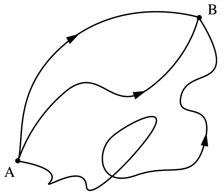
This picture shows an electron that was observed at A at time $t_1$ and then at B at time $t_2$ . In the quantum picture, the electron could have taken any path from A to B. Each of these paths are associated with a probability.

When we ask the question: What is the probability that the electron will be at B at time $t_2$ , we sum up the probability amplitudes corresponding to all these paths to arrive at an answer.

We could just as well ask : What is the probability that the electron will be at B at time $t_2$ and the proper time shown by the clock that the electron carries will read $\tau$ at that instant? This is a perfectly valid question and has a different answer from the question asked previously.

The proper time at the point B is a dynamical variable now, which depends on the path chosen. Therefore, it could have a whole range of values, thereby proving that it is indeed an observable.

To calculate this probability, we need to sum up the probability amplitude corresponding only to those paths that will make the proper time read $\tau$ and ignore the other paths altogether.

Conceptually okay, mathematically …

At first sight, this seems to be an interesting way of including time as an observable. The salient points are summarized here:

We use proper time as a time variable that is observable.
Instead of asking only about position of a particle, we ask about position and proper time of a particle.
There seems to be a way to calculate probabilities of measuring the above information from the Feynman Path Integral picture of QM.
The time variable in question is now a property of the particle, just like position, momentum and energy.
In an $N$ particle system, we will have to deal with $N$ time variables and $3N$ space variables.
There is one conceptual shortcoming: proper time and space do not make up a four vector like momentum and energy.

I will attempt a calculation of the above mentioned probability, and if I get something, I will post the results here.

Identity crisis

July 1, 2015July 3, 2015 dibya2 Comments

Quantum mechanics is simple

Quantum Mechanics is conceptually simple. To describe a physical situation and compute its evolution Quantum Mechanically, one needs only two pieces of information:

The complete set of commuting observables
The Hamiltonian

The rest is just a matter of doing the math right!

Relativistic QM is also simple, but the identity operator changes

Same is the story of relativistic Quantum Mechanics, which is conceptually quite similar to its non relativistic variant. However, the move to four dimensions and the existence of Lorentz Invariance (LI) in four dimensions introduces a few natural changes to the mathematical apparatus.

One such change occurs in the familiar identity operator of Quantum Mechanics. In this post, I wish to discuss the changes to the identity operator when the physical situation involves relativistic spinless particles.

What’s so special about the identity operator?

The identity operator appears everywhere in QM. Almost any computation you’ll ever do will have the identity operator somewhere in it. It is therefore definitely special and we should know how it changes in the relativistic case.

There are some other compelling reasons to study it too:

The modified identity operator gives us the relativistic normalization condition.
This trick could be generalized to other symmetries to quickly derive the normalization condition for that symmetry.
It illustrates an interesting difference between position space and momentum space in Relativistic QM and raises some difficult conceptual questions.

Are you ready? 😉 Here we go.

Key difference: kets now represent 4 dimensional momentum

The major change that happens when we shift from 3 dimensions to 4 dimensions is that all the physical quantities become 4 dimensional too. Ditto for momentum.
Therefore the ket $\left|{k}\right>$ now represents $\left|k^0, k^1, k^2, k^3\right>$ , not $\left|k^1, k^2, k^3\right>$ .

Finding the identity operator by analogy
In 3 Dimensions, the identity operator was:

$I = \int{d^{3}k \left|k^1, k^2, k^3\right>\left<k^1, k^2, k^3\right|}$

The four dimensional analog seems to be:

$I = \int{d^{4}k \left|k^0, k^1, k^2, k^3\right>\left<k^0, k^1, k^2, k^3\right|}$

Get rid of the non physical states

The last expression is grossly incorrect because many of the states in the above integral are not physical. Remember the relativistic constraints $k^0 > 0$ and $k^2 = m^2$ , where $m$ is the rest mass of the particle in question? Only states that satisfy these constraints are physical and should be kept in the integral. The rest of the states should be omitted as they are irrelevant to physics.

The mathematical trick to include only physical states is simple. We multiply the integral by the correct Delta function $\delta(k^2 - m^2)$ and the Heaviside step function $\theta(k^0)$ .

$I = \int{d^{4}k\delta(k^2 - m^2) \theta(k^0) \left|k^0, k^1, k^2, k^3\right>\left<k^0, k^1, k^2, k^3\right|}$

and we obtain the correct identity operator for Relativistic Quantum Mechanics, which is:

$I = \int{ \frac{d^{3}k}{2\sqrt{\vec{k}^2 + m^2}} \left|k^1, k^2, k^3\right>_R\left<k^1, k^2, k^3\right|_R}$

which is often written like

$I = \int{ \frac{d^{3}k}{2 \omega_{\vec{k}}} \left|\vec{k} \right>_R\left<\vec{k}\right|_R}$

where the subscript $R$ denotes physical relativistic momentum eigenkets that have the correct energy momentum relation. $\omega_{\vec{k}}$ is the energy of a particle with the three momentum $\vec{k}$ .

Normalization

From the identity operator, one can immediately conclude the following:

$\left<\vec{k^{\prime}} | \vec{k} \right>_R = 2 \omega_{\vec{k}} \delta^3 (\vec{k^{\prime}} - \vec{k})$

and voila! We have the correct relativistic normalization of momentum eigenkets.

The problem with the position space and relativistic Quantum mechanics

The procedure mentioned in this post is so simple and straightforward, that one cannot help wondering: can we do the same with position eigenkets? That is, can we express the relativistic identity operator in terms of position eigenkets?

We can naively follow the analogy between 3 and 4 dimensions and arrive at the following equation:

$I = \int{d^{4}x \left|x^0, x^1, x^2, x^3\right>\left<x^0, x^1, x^2, x^3\right|}$

Of course, this expression is grossly incorrect once again. There are two important things that one needs to consider:

We know that the identity operator in 3 dimensions include positions eigenkets that correspond to the same time. However the expression “same time” is observer dependent in relativity. Therefore this integral needs to constrained to 4 dimensional eigenkets corresponding to the same time, as measured by a specific observer.
Also it is somewhat unclear whether to include pairs of 4 dimensional eigenkets that are separated by space like 4 vectors.

The best one can do, therefore, is to construct observer dependent identity operators, which isn’t such a good idea.

The difference between position and momentum space

I want to end this post by trying to understand the difference between the momentum and the position space, which made it impossible to construct a relativistic identity operator based on position space eigenkets.

It seems that the difference lies in the additional constraint that we had to impose in the case of the position space construction. This was the constraint of same time. This constraint is not Lorentz Invariant and therefore we ran into a problem.

We must remember that the constraint of same time is key in non relativistic Quantum Mechanics and it does not generalize well in the Relativistic variant. Why is that?? This is an open question and I do not know any satisfying answer to why this happens.

The crazy system of units in particle physics

June 3, 2015July 1, 2015 dibyaLeave a comment

The system of units

Particle physicists routinely say things like the following:

The mass of an Electron is $0.5 \text{ MeV}$
The Compton wavelength of a Proton is $1 \text{ GeV}^{-1}$

This doesn’t make a lot of sense at first sight. The unit of mass was supposed to be kilograms, not $\text{MeV}$ . The unit of length was supposed to be meters, not $\text{ GeV}^{-1}$ . So, what’s happening here?

MeV and GeV are units of energy

The energy of an Electron that travels through a potential difference of 1 Volt starting from rest is 1 eV.

Both MeV and GeV ( $10^6 \text{ eV} = 1 \text{ MeV} \text{ and } 10^9 \text{ eV} = 1 \text{ GeV}$ ) are therefore units of energy.
Particle physicists love expressing all physical quantities in terms of energy. But the funny thing is, this is actually impossible. Length cannot be expressed in terms Energy alone.
How do they do it then? It turns out that they have invented a slang that makes the impossible possible. All we need to do is to understand how their slang works.

The relation of energy and other physical quantities

Mass, time and length are, of course, related to energy. Energy has the following dimension: $[E] = \frac{[M][L]^{2}}{[T]^{2}}$ . If we divide energy by velocity squared, we are left with mass. Thus $\frac{\text{MeV}}{c^2}$ is an unit of mass. Similarly, angular momentum divided by energy gives us time. Thus $\frac{\hbar}{\text{GeV}}$ gives us the unit of time. Going one more step further, $\frac{\hbar}{\text{GeV}}\times c$ gives us the unit of length.

Particle Physics slang

The important thing to realize is that units in Particle Physics are not really units, they are more like a slang. A common language that they understand but you don’t.

When they say the mass of an Electon is $0.5 \text{ MeV}$ , they really mean $0.5 \frac{\text{MeV}}{c^2}$ . When they say the Compton wavelength of a Photon is $1 \text{ GeV}^{-1}$ , they really mean $1 \frac{\hbar}{\text{GeV}}\times c$ .
They are simply omitting the $\hbar$ and the $c$ , but they are always there. It is your job to add the correct multiplicative factor to what they are saying.
For mass, the factor is $\frac{1}{c^2}$ , for time it is $\hbar$ , for length, it is $\hbar \times c$ .

What about velocity and angular momentum?

One cannot go from energy to velocity or angular momentum by multiplying or dividing by powers of $\hbar$ or $c$ . You can try it, it is plain impossible.
The procedure that makes sense for these two physical quantities is as follows: Speak of velocity and angular momentum as if they are dimensionless. This is, of course, the slang. To convert the slang to High Physics always multiply all velocities by $c$ and all angular momentum by $\hbar$ .

What’s so special about $c$ and $\hbar$ ?

Absolutely nothing. They are just two of the many universal constants in Physics. One could make up another slang by choosing the universal gravitational constant $G$ and the speed of light $c$ and using multiplicative factors involving them. In this new slang, we’d say:

The mass of an Electron is $0.5 \text{ MeV}$
The Compton wavelength of the same Proton is now $10^{39} \text{ GeV}$ (the multiplicative factor being $\frac{G}{c^5}$ )
The speed of light is 1
The universal constant of Gravitation is also 1
The Planck constant is approximately $10^{39} \text{ GeV}^2$ (the multiplicative factor being $\frac{G}{c^5}$ )

expploration

explore the world of elementary particle physics